Vertical grid (vgrid.in)

See Numetical Formulation chapter for details of different types of vgrid supported in SCHISM. Following are a few example vgrid.in.

An example of SZ grid

2 !ivcor (1: LSC2; 2: SZ)
54 18 100. !nvrt(=Nz); kz (# of Z-levels); hs (transition depth between S and Z)
Z levels !Z-levels in the lower portion
1 -5000. !level index, z-coordinates
2 -2300.
3 -1800.
4 -1400.
5 -1000.
6 -770.
7 -570.
8 -470.
9 -390.
10 -340.
11 -290.
12 -240.
13 -190.
14 -140.
15 -120.
16 -110.
17 -105.
18 -100. !z-coordinate of the last Z-level must match -h_s
S levels !S-levels below
30. 0.7 10. ! constants used in S-transformation: hc, theta_b, theta_f
18 -1.
 !first S-level (sigma-coordinate must be -1)
19 -0.972222
 !levels index, sigma-coordinate
20 -0.944444
.
.
.
54 0.
 !last sigma-coordinate must be 0

Notes: - The water column is from the bottom (kbp, variable in space) to surface (level nvrt) at each node; - The code will crash if the surface elevation falls below \(–h_c\) so make sure \(h_c\) is sufficiently large (there is a hardwired lower bound for this around 5m in the code).

An example of pure S grid

If a "pure S" model is desired, use only 1 Z-level and set hs to a very large number (e.g., 1.e6) above. For example, using vgrid.in below leads to a 2D model.

2 !ivcor
2 1 1.e6
Z levels
1 -1.e6
S levels
40. 1. 1.e-4
1 -1.
2 0.

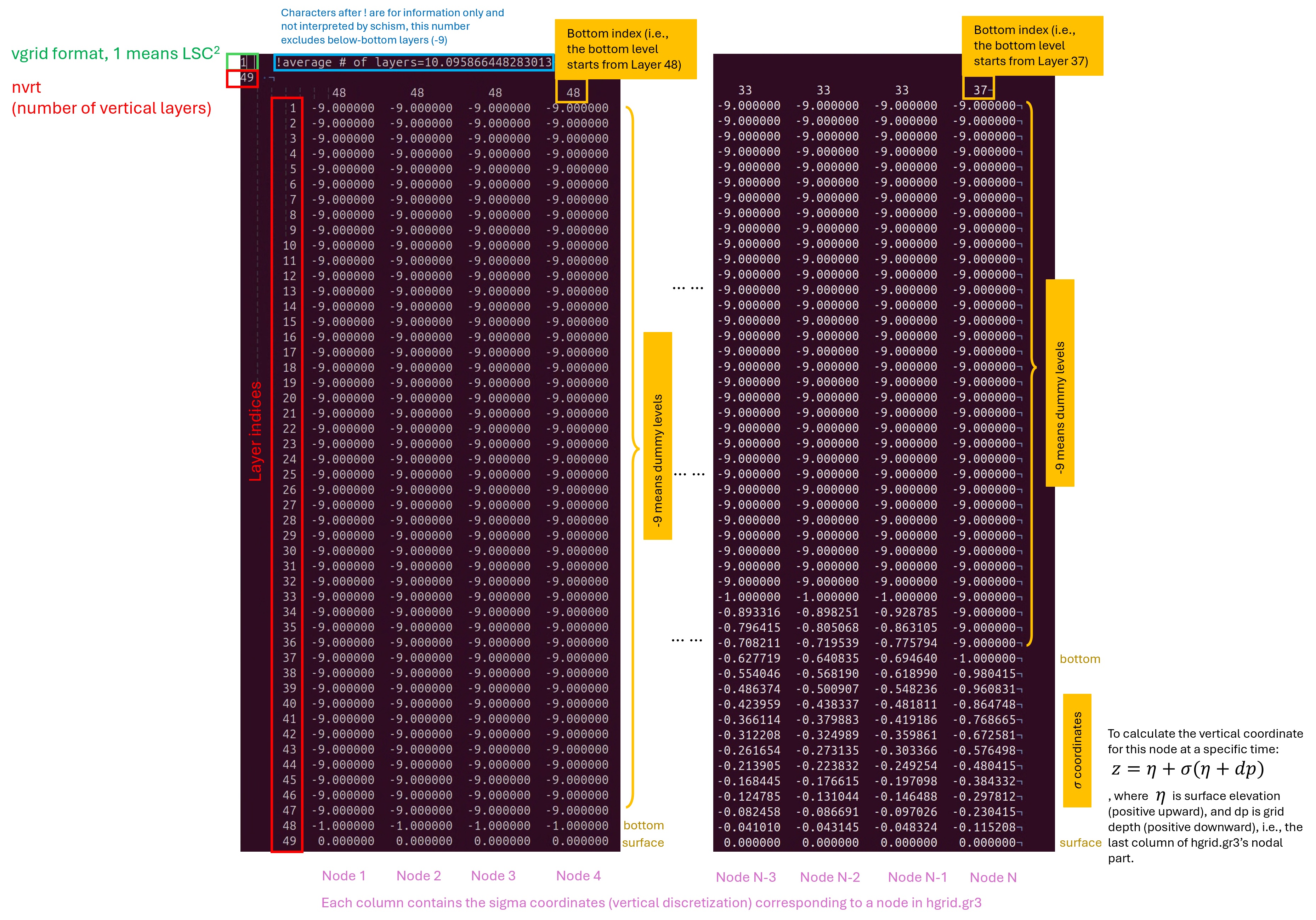
An example of \(LSC^2\) grid

This type of grid requires some user experience and can be generated using scripts (e.g., Utility/Pre-Processing/gen_vqs*.f90). There is no limit such as \(h_c\) mentioned above, so \(LSC^2\) is more robust.

1 !ivcor (1: LSC2; 2: SZ)
39 !nvrt(=Nz)
10 4 4 4 4 10 4 10 10 ...  !bottom level indces at all nodes
1 -1. -1. -1. -1. -9. -9. -9. ... !level #, sigma coordinates $\in [-1,0]$ at level 1 for all nodes. '-9' means level 1 is below the bottom of this node
2 -0.884251  -0.874424  -0.888763 -0.884930 -1. ...