Case studies

Hydrologic flow

Simulation of hydrologic flow in watershed, with bottom elevation above sea level (thus strong wetting and drying) and with complex river channel network, is challenging. The discussions below are taken from a training course on compound flooding simulation.

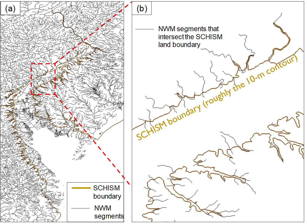
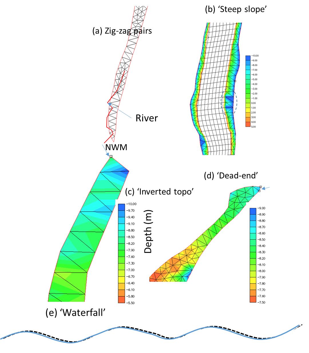
A common, convenient method for introducing river flows into watershed in SCHISM mesh is via the point source/sinks as shown in Figure 8. Together with proper parameter choices (e.g., a small minimum depth of 10-5m, a fully implicit scheme, a large bottom friction with proper vertical grid to allow for 2D representation in the watershed etc) this usually works fine for smaller rivers. For large rivers, the open-boundary approach (i.e., river channels as open boundary segments) is the preferred method. In general, the point source approach injects flow via the continuity equation alone without providing extra momentum (note that the volume sources/sinks are added to the RHS of Eqs. 2 and 3 but not in the momentum Eqs. 1, and thus it will take the system some time to adjust internally to set up the flow from the pressure gradient. Because of this drawback, large elevations may be found near the injection points, especially during initial ramp up or during high and rapidly varying flow periods. This symptom can be exacerbated by the following missteps:

1. Pairs of source and sink in close proximity (Figure 9a). Users should combine these pairs;
2. Steep slopes near boundary with coarse resolution (Figure 9b);
3. Inverted bed slopes near the injection location (so the flow has to overcome gravity; Figure 9c);
4. Poorly ventilated ‘dead-end’ (Figure 9d);
5. Undulating channel (‘water fall’; Figure 9e).

The model is stable, but interpretation of results may be problematic in those cases. Besides more grid work in those spots, using open-boundary segments can help. Also one should really exclude transient responses during ramp-up period in computing the maximum elevation to allow the system time to adjust. Also don’t forget that sometimes the rainfall (which can also be introduced as sources) on high mountains should result in high surface elevations there, which are realistic.

To get accurate results in the hydrologic regime, it is also important to resolve channels to avoid blocking flows. Semi-automatic mesh generation tools have been developed specifically for this purpose; see this chapter.

Coupling of hydrologic model (National Water Model in this case) with SCHISM. The river network (lines) intersects SCHISM land boundary, and the river flow is introduced at the intersection points (sources for inflow and sinks for outflow).

Pathologic cases for hydrologic flows.

Tsunami simulations

Your can diwnload a sample tsunami run (impact of Alaska tsunami waves on Cannon Beach, OR) at http://www.ccrm.vims.edu/yinglong/wiki_files/tsunami_ex15.tgz

Note that the files are compatible with the serial version of SCHISM, but the idea for parallel version is similar.

The operational time step for tsunami applications is generally in the range of a few seconds because of the constraint from shorter wavelength and inundation processes. You'll need higher mesh resolution also to satisfy the inverse CFL criterion (CFL>0.2). The inundation results may also be sensitive to the min. depth used in the run (1cm in this example). If you use the newer parallel version, you can also use a 2D model with a proper Manning coefficient.

Typically you need to follow these 2 steps in tsunami simulations:

1. Deformation run (EX15/Def/ in the sample run): this simulates the earthquake and the set-up of the initial surface waves. For this you need:

     a) `bdef.gr3` (refer to the user manual) which specifies the total seafloor deformation.
     b) turn on the hotstart output handle, and `dt=1s, ibdef=10, rnday=1.158e-4`
     c) We typically run this stage for 10 sec duration and at the end of the run you'll find an output files called `10_hotstart` which is then used as hotstart.in for the next (propagation and inundation) stage.
     d) In addition, use `mod_depth.f` (inside the bundle), which takes info in `bdef.gr3` and `hgrid.gr3` (pre-earthquake depths) to generate hgrid.new (post-earthquake depths). The latter is used in the next stage. For completeness you need to attach the boundary condition part (`b.tmp` in the bundle) of `hgrid.gr3` to the end of `hgrid.new`;
   

2. Propagation and inundation stage (EX15/ in the sample run): this run continues from the deformation run above with no further seafloor movement. You'll notice that many input files are identical to the Def/ run, but be careful of differences in hgrid.gr3 (linked to Def/hgrid.new) and param.in (imm=0 etc).

     a) For this run we also turn off the advection in the open ocean (up to say 60m isobath) because it's negligible there (`adv.gr3`) -  this bypasses the inverse CFL criterion and allows you to use a coarser resolution in deeper ocean.
     b) Also note that `hotstart.in` is from the previous stage. 
   

3. After the run is done you can look at global outputs (elevation, depth-averaged velocity etc). The maximum elevation (maxelev.gr3) and depth-averaged velocity (maxdahv.gr3) are also part of the outputs (for parallel versions, use /src/Utility/Combining_Scripts/combine_gr3.f90). The maximum inundation can be easily computed from maxelev.gr3.