Visualization

Visualization with Matlab¶

The directory Utility/Vis_Matlab/ has matlab scripts that can visualize outputs along a horizontal slab (at a fixed z level or at a sigma level) or vertical transects. In particular, SCHISM_SLAB2.m and SCHISM_TRANSECT2.m for for the new scribed outputs, while SCHISM_SLAB.m and SCHISM_TRANSECT.m are for the old outputs (schout*.nc).

Visualization with pylib¶

pylib provides schismview to visualize outputs (scribed outputs, OLDIO not supported yet). schismview will collect all the available variables from your outputs. For each variable, you can do 1). contour plot, 2). animation, 3). extract time series, and 4) query, etc. This is a lightweight app, and please report bug to SCHISM maillist or wzhengui@gmail.com.

Installation of pylib¶

By running the following code, you can locate the executable of schismview
python -c "from pylib import *; print(mylib.__file__[:-16]+'Scripts/schismview')"

How to use `schismview`¶

To lauch schismview, you can run the executable either under your run directory, or pass the run directory as a argument to the executable, which will give you an schismview window below.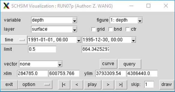
variable: All availalbe SCHISM output variables are collected, and you can choose the variable you want to view from the list window.
figure: list of figures. You can have multiple figures for different variables. You can close it if you want. Later on, you can retrieve previous figures from the list. If you want to add a new figure, choose add.
layer: For 3D variable, you can specify which layer you want to view. For 2D variable, this option is not needed.
grid or bnd: If clicked, schism grid/boundary will plotted out along with the contour plot. If you only want to view the grid/boundary, choose none from the variable list.
ctr: By default, schismview will use tripcolor to plot contours, which is element-based. If ctr is clicked, schismview will use tricontourf to plot, which can be faster for very large grid.
time: There are three available time options (calendar time, SCHISM stack number, or Julian date). You can set the Start and End dates for viewing variables in the textbox. This may be needed for animation if you only want to view for a specific period of time.
limit: It sets the lower and upper limits of contours. The values beyond are extended.
vector: You can choose vector you want to view from the list. vector shown will be limitted to the current domain specified by xlim and ylim.
curve: By right double click, you can add location points for extractng times for the active variable. middle double click will remove the points. Then, click curve, schismview will extract time series in background and the button will display wait. Once wait becomes curve again, clicking on it will show the time series. Note, extracting time series can be very slow for 3D variables depending on how the netcdf outputs are stored (chuncking the files can help, but it is a separate topic beyond schismview). It is better to specify short time range.
query: You can query the value of variable. By clicking query (becomes sunken once chosen), you can use middle single click to query the value. By clicking query again, it will exit query mode.
xlim/ylim: Sspecify the X/Y axis range.
animation
- |<: go to start time
- <: go to previous time
- play: play animation for the current variable. The button will display stop, and click stop will stop the animation. Note doulbe right click will have the same effect of play buttion
- >: go to next time
- >|: go to end time
- skip: specify the animation interval
draw: draw plot or refresh the plot.
option: Advaned features
- command window: type commands to interact with the plot, which can be used to generate desired high-quality figures.
- save animation
- show node/element number

Visualization with VisIt¶

The most comprehensive way to visualize SCHISM nc4 outputs is via VisIt.

Shortly after v5.9.0, we have successfully implemented a new mode of efficient I/O using dedicated 'scribes'. At runtime, the user needs to specify number of scribe cores (= # of 3D outputs variables (vectors counted as 2) plus 1), and the code, compiled without OLDIO, will output combined netcdf outputs for each 3D variable and also all 2D variables in out2d*.nc. Sample 3D outputs are: salinity_*.nc, horizontalVelX_*.nc etc - note that vectors variable names end with X,Y. You can find sample outputs here. Sample outputs using OLDIO (schout*.nc) can be found here.

You can download newer versions of VisIt plugins c/o Jon Shu, DWR by following these steps:

On Windows 7 or 10

First download VisIt from LLNL site and install. Note the location, which will be in your Windows profile directory if you install for the current user or in Program Files if you install for all users. Note the location.
Make sure MS visualc++ 2012 x64 is installed. If not, google it and install and restart (this is required for using multi-core VisIt). If you are using VisIt 3.3.1, you need MS visualc++ 2013 x64 also.
Download pre-built plug-in, developed at California Dept of Water Resource
You need to put the plugin dlls in: %USERPROFILE%\Documents\VisIt\databases (create new folders if necessary), except netcdf_c++.dll. The NetCDF DLL needs to be copied to the VisIt installation directory, which may be %USERPROFILE%\LLNL\VisIt 3.3.1 if you installed for yourself or the system install directory C:Program Files\LLNL\VisIt3.3.1. if you installed for all users.
After these steps, you should be able to read in SCHISM outputs in ViSIt; look for SCHISM, gr3 format from the dropdown list. To load in vectors, select only the X file.

On Linux Systems

Newer versions can be found at the master branch of github.

Note

Note that the new plugins also work with the old I/O (combined schout*.nc) or even the older binary outputs. To visualize any variables under new I/O with VisIt, you'll always need corresponding out2d*.nc; additionally for any 3D variables, VisIt also needs corresponding zCoordinates*.nc.