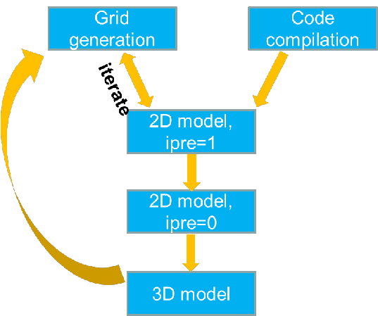
Typical workflow (a cheat sheet)
Mesh generation tips
- Generate meshes in map projection, not lon/lat; this gives flexibility of setting element size (although newer SMS versions can now handle distance in lon/lat directly). Distortion due to projection can be rectified later by projecting back to lon/lat;
- Make sure major channels are resolved with at least 1 row of ‘always wet’ elements – no blockage of major channel flow
- Always keep the map file and DEM sources and be willing to edit the grid, as often the model results (and sometimes performance) depend on the mesh
- Being an implicit model with ELM treatment of momentum advection, SCHISM has an
operating rangefor the time step. For field applications, the range is 100-400 sec for barotropic cases, 100-200 sec for baroclinic cases. If you have to reduce the time step, make sure you recheck the inverse CFL criterion again. - First estimate the smallest \(\Delta t\) you’d anticipate (e.g., 100s for field applications), and then estimate the coarsest \(\Delta t\) at sample depths to make sure \(CFL>0.4\) (cf. Table 5.1).
- Resolving features is much easier with SCHISM – be game! Bathymetry smoothing is not necessary.
- Make sure open boundaries do not become completely dry during simulation
- [3D simulations with transport] Implicit \(TVD^2\) transport is very efficient, but horizontal transport is still explicit
(and is the main bottleneck). Therefore beware of grid resolution in critical regions to avoid
excessive sub-cycling; use upwind in areas of no stratification. Another way to speed up is
to use hybrid ELM and FV by setting
ielm_transport=1. - Check the following things immediately after a mesh is generated (via ACE/xmgredit5 or scripts)
- Minimum area: make sure there are no negative elements (under xmgredit5->Status).
- \(CFL>0.4\) (at least in ‘wet’ areas). Note that you need to do this check in map projection (meters), not in lon/lat!
- Maximum skewness for triangle: use a generous threshold of 17, mainly to find excessive "collapsed" elements that originate from the SMS map issues (and fix them in SMS).
- As a general rule of thumb, SCHISM can comfortably handle elements >= \(1m^2\) (\(10^{-10}\) in lon/lat), and skewness<=60. Use
ACE/xmgredit5or SMS to check these. Most of those extreme elements are due to SMS map issues so you should fix them there. - Fix bad quads: fix all bad-quality quads using
fix_bad_quads.f90as the last step; use 0.5 (ratio of min and max internal angles) as threshold.
2D model: pre-processing
- Check additional grid issues with a 2D barotropic model with
ipre=1,ibc=1,ibtp=0- You can cheat without any open boundary segments during this step
- Remember to
mkdir outputsin the run directory
- Iterate with mesh generation step to fix any mesh issues.
2D model: calibration
- Start from simple and then build up complexity. Simplest may be a tidal run with a constant Manning’s \(n\).
- Remember most outputs are on a per-core basis if you use OLDIO and need to be combined using the
utility scripts; e.g., for global outputs (schout*.nc), use
combine_output11.f90to get global netcdf outputs that can be visualized by VisIT or other tools; for hotstart, usecombine_hotstart7.f90. If you use new scribe I/O, you don't need to combine global outputs, but still need to combine hotstart outputs. - Examine surface velocity in animation mode to find potential issues (e.g. blockage of channels)
- Negative river flow values for inflow
- Check all inputs: ‘junk in, junk out’. There are several pre-processing scripts for this purpose. Xmgredit5 or SMS is very useful also.
3D model: calibration
- The model may need velocity boundary condition at ocean boundary. The easiest approach is to
use FES2014 or TPXO tide package to generate tidal velocity, and use a global ocean model (e.g. HYCOM) to get sub-tidal velocity. Then use type ‘5’ in
bctides.in. - Avoid large bottom friction in shallow areas in 3D regions
- Examine surface velocity in animation mode to find potential issues
- Control the balance between numerical diffusion and dispersion (
indvel,ihorcon) - Transport solver efficiency may require some experience.
- \(LSC^2\) grid requires some learning/experience, but is a very powerful tool (resembling unstructured grid in the vertical)
- See Case studies for commonly encountered issues in 3D setup.
Note
Another good resource for beginners is a mini live manual by Ms. Christelle Auguste (U. of Tasmania). There is a PDF on there.