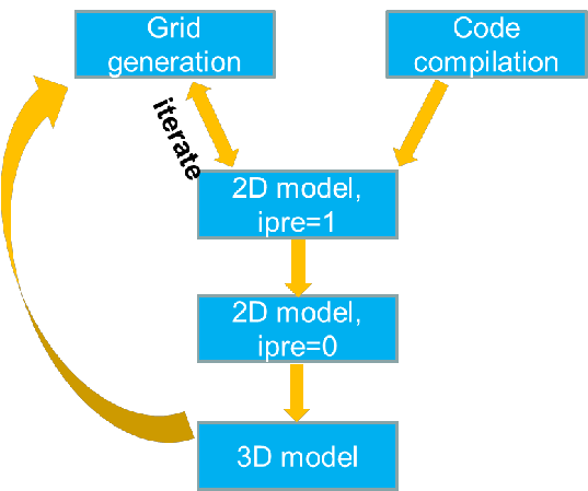
Typical workflow (a cheat sheet)

Grid generation¶

Generate grids in map projection, not lon/lat. Gives flexibility of setting element size.
Make sure major channels are resolved with at least 1 row of ‘always wet’ elements – no blockage of major channel flow
Always keep the map file and DEM sources and be willing to edit the grid, as often the model results (and sometimes performance) depend on the grid
Being an implicit model with ELM treatment of momentum advection, SCHISM has an operating range for the time step. For field applications, the range is 100-400 sec for barotropic cases, 100-200 sec for baroclinic cases. If you have to reduce the time step, make sure you recheck the inverse CFL criterion as show below.
First estimate the smallest \(\Delta t\) you’d anticipate (e.g., 100s for field applications), and then estimate the coarsest \(\Delta t\) at sample depths to make sure \(CFL>0.4\) (cf. Table 5.1).
Resolving features is much easier with SCHISM – be game! Bathymetry smoothing is not necessary.
Make sure all open boundaries stay wet during simulation. This condition has been relaxed from v5.8 but the code will still crash when an entire open boundary segment is dry.
Implicit \(TVD^2\) transport is very efficient, but horizontal transport is still explicit (and is the main bottleneck). Therefore beware of grid resolution in critical regions to avoid excessive sub-cycling; use upwind in areas of no stratification.
Check the following things immediately after a grid is generated (via ACE/xmgredit5)
- \(CFL>0.4\) (at least in ‘wet’ areas). Note that you need to do this check in map projection (meters), not in lon/lat!
- Minimum area: make sure there are no negative elements.
- Maximum skewness for triangle: use a generous threshold of 13, mainly to find excessive "collapsed" elements.
- Quad quality: use 0.5 (ratio of min and max internal angles) as threshold.

2D model: pre-processing¶

Check additional grid issues with a 2D barotropic model with ipre=1, ibc=1, ibtp=0
- You can cheat without any open boundary segments during this step
- Remember to mkdir outputs in the run directory
Iterate with Grid generation step to fix any grid issues.

2D model: calibration¶

Start from simple and then build up complexity. Simplest may be a tidal run with a constant Manning’s \(n\).
Remember most outputs are on a per-core basis if you use OLDIO and need to be combined using the utility scripts; e.g., for global outputs (schout*.nc), use combine_output11.f90 to get global netcdf outputs that can be visualized by VisIT; for hotstart, use combine_hotstart7.f90.
Examine surface velocity in animation mode to find potential issues (e.g. blockage of channels)
Negative river flow values for inflow
Check all inputs: ‘junk in, junk out’. There are several pre-processing scripts for this purpose. Xmgredit5 or SMS is very useful also.

3D model¶

The model needs velocity boundary condition at ocean boundary. There are two alternative approaches for this:
- Use FES2014 tide package to generate tidal velocity, and use a global ocean model (e.g. HYCOM) to get sub-tidal velocity. Then use type ‘5’ in bctides.in.
- Use the one-way nesting capability to generate velocity boundary condition at the ocean boundary. You may use the 2D barotropic tidal model for this purpose, and then augment the tidal velocity with baroclinic velocity from a large-scale model like HYCOM.
Avoid large bottom friction in shallow areas in 3D regions
Examine surface velocity in animation mode to find potential issues
Control the balance between numerical diffusion and dispersion (indvel, ihorcon)
Transport solver efficiency may require some experience.
\(LSC^2\) grid requires some learning/experience, but is a very powerful tool (resembling unstructured grid in the vertical)
See Case studies commonly encountered issues in 3D setup.

Note

Another good resource for beginners is a mini live manual written on Overleaf by Ms. Christelle Auguste (U. of Tasmania).